Consider a model with parameters $\theta$ and latent variables $\mathbf{Z}$; the expectation-maximization algorithm (EM) is a mechanism for computing the values of $\theta$ that, under this model, maximize the likelihood of some observed data $\mathbf{X}$.

The joint probability of our model can be written as follows:

$$ p(\mathbf{X}, \mathbf{Z}\vert \theta) = p(\mathbf{X}\vert \mathbf{Z}, \theta)p(\mathbf{Z}\vert \theta) $$

where, once more, our stated goal is to maximize the marginal likelihood of our data:

$$ \log{p(\mathbf{X}\vert\theta)} = \log{\sum_{\mathbf{Z}}p(\mathbf{X, Z}\vert\theta)} $$

An example of a latent variable model is the Latent Dirichlet Allocation¹ (LDA) model for uncovering latent topics in documents of text. Once finished deriving the general EM equations, we'll (begin to) apply them to this model.

Why not maximum likelihood estimation?

As the adage goes, computing the MLE with respect to this marginal is "hard." For one, it requires summing over an (implicitly) humongous number of configurations of latent variables $z$. Further, as Bishop² states:

A key observation is that the summation over the latent variables appears inside the logarithm. Even if the joint distribution $p(\mathbf{X, Z}\vert\theta)$ belongs to the exponential family, the marginal distribution $p(\mathbf{X}\vert\theta)$ typically does not as a result of this summation. The presence of the sum prevents the logarithm from acting directly on the joint distribution, resulting in complicated expressions for the maximum likelihood solution.

We'll want something else to maximize instead.

A lower bound

Instead of maximizing the log-marginal $\log{p(\mathbf{X}\vert\theta)}$ (with respect to model parameters $\theta$), let's maximize a lower-bound with a less-problematic form.

Perhaps, we'd work with $\log{p(\mathbf{X}, \mathbf{Z}\vert \theta)}$ which, almost tautologically, removes the summation over latent variables $\mathbf{Z}$.

As such, let's derive a lower-bound which features this term. As $\log{p(\mathbf{X}\vert\theta)}$ is often called the log-"evidence," we'll call our expression the "evidence lower-bound," or ELBO.

Jensen's inequality

Jensen's inequality³ generalizes the statement that the line secant to a concave function lies below this function. An example is illustrative:

png

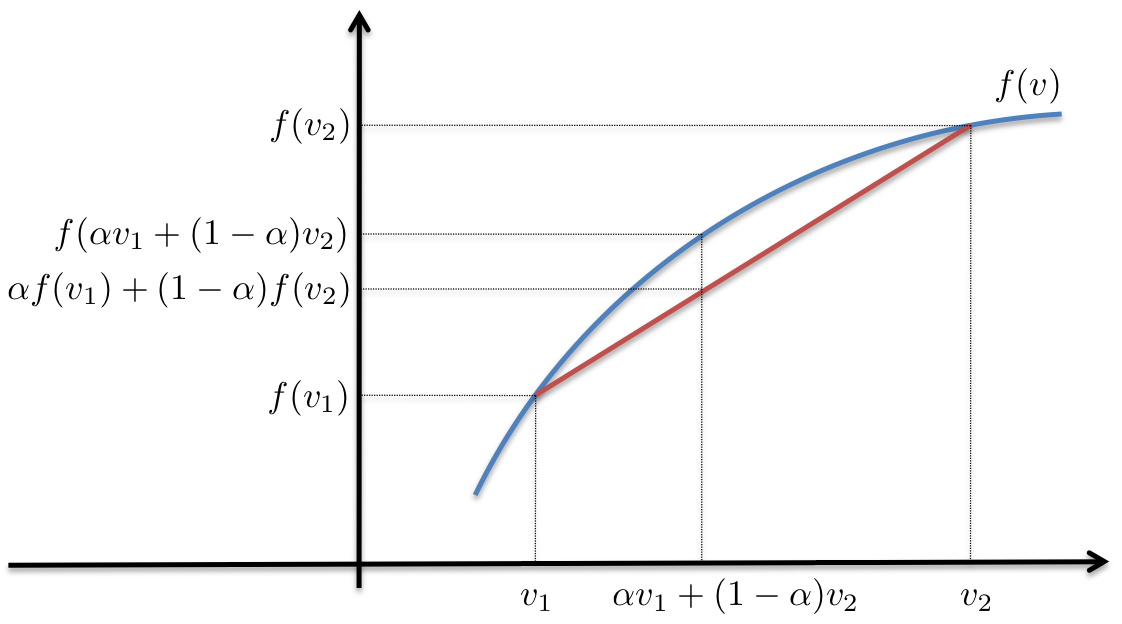
First, we note that the red line is below the blue for all points for which it is defined.

Second, working through the example, and assuming:

$f(x) = \exp(-(x - 2)^2)$
$v_1 = 1; v_2 = 2.5; \alpha = .3$

$$ \begin{align*} f(v_1) &\approx .3679\\ f(v_2) &\approx .7788\\ \alpha f(v_1) + (1 - \alpha)f(v_2) &\approx \bf{.6555}\\ \end{align*} $$

$$ \begin{align*} \alpha v_1 + (1 - \alpha)v_2 &= 2.05\\ f(\alpha v_1 + (1 - \alpha)v_2) &\approx \bf{.9975}\\ \end{align*} $$

we see that $\alpha f(v_1) + (1 - \alpha)f(v_2) \leq f(\alpha v_1 + (1 - \alpha)v_2)$.

Finally, we arrive at a general form:

$$ \mathop{\mathbb{E}_{v}}[f(v)] \leq f(\mathop{\mathbb{E}_{v}}[v]) $$

where $p(v) = \alpha$.

Deriving the ELBO

In trying to align $\log{p(\mathbf{X}\vert\theta)} = \log{\sum\limits_{\mathbf{Z}}p(\mathbf{X, Z}\vert\theta)}$ with $f(\mathop{\mathbb{E}_{v}}[v])$, we see a function $f = \log$ yet no expectation inside. However, given the summation over $\mathbf{Z}$, introducing some distribution $q(\mathbf{Z})$ would give us the expectation we desire.

$$ \begin{align*} \log{p(\mathbf{X}\vert\theta)} &= \log{\sum_{\mathbf{Z}}p(\mathbf{X, Z}\vert\theta)}\\ &= \log{\sum_{\mathbf{Z}}q(\mathbf{Z})\frac{p(\mathbf{X, Z}\vert\theta)}{q(\mathbf{Z})}}\\ &= \log{\mathop{\mathbb{E}}_{q(\mathbf{Z})}\bigg[\frac{p(\mathbf{X, Z}\vert\theta)}{q(\mathbf{Z})}}\bigg]\ \end{align*} $$

where $q(\mathbf{Z})$ is some distribution over $\mathbf{Z}$ with parameters $\lambda$ (omitted for cleanliness) and known form (e.g. a Gaussian). It is often referred to as a variational distribution.

From here, via Jensen's inequality, we can derive the lower-bound:

$$ \begin{align*} \log{p(\mathbf{X}\vert\theta)} = \log{\mathop{\mathbb{E}}_{q(\mathbf{Z})}\bigg[\frac{p(\mathbf{X, Z}\vert\theta)}{q(\mathbf{Z})}\bigg]} &\geq \mathop{\mathbb{E}}_{q(\mathbf{Z})}\bigg[\log{\frac{p(\mathbf{X, Z}\vert\theta)}{q(\mathbf{Z})}}\bigg]\\ &= \mathop{\mathbb{E}}_{q(\mathbf{Z})}\bigg[\log{\frac{p(\mathbf{X, Z}\vert\theta)}{q(\mathbf{Z})}}\bigg] + R \end{align*} $$

Et voilà, we see that this term contains $\log{p(\mathbf{X, Z}\vert\theta)}$; the ELBO should now be easier to optimize with respect to our parameters $\theta$.

So, what's $R$?

$$ \begin{align*} R &= \log{p(\mathbf{X}\vert\theta)} - \mathop{\mathbb{E}}_{q(\mathbf{Z})}\bigg[\log{\frac{p(\mathbf{X, Z}\vert\theta)}{q(\mathbf{Z})}}\bigg]\\ &= \log{p(\mathbf{X}\vert\theta)} - \mathop{\mathbb{E}}_{q(\mathbf{Z})}\bigg[\log{p(\mathbf{X, Z}\vert\theta) - \log{q(\mathbf{Z})}}\bigg]\\ &= \log{p(\mathbf{X}\vert\theta)} - \mathop{\mathbb{E}}_{q(\mathbf{Z})}\bigg[\log{p(\mathbf{Z}\vert\mathbf{X}, \theta)} + \log{p(\mathbf{X}\vert\theta)} - \log{q(\mathbf{Z})}\bigg]\\ &= \mathop{\mathbb{E}}_{q(\mathbf{Z})}\bigg[\log{p(\mathbf{X}\vert\theta)}\bigg] - \mathop{\mathbb{E}}_{q(\mathbf{Z})}\bigg[\log{p(\mathbf{Z}\vert\mathbf{X}, \theta)} + \log{p(\mathbf{X}\vert\theta)} - \log{q(\mathbf{Z})}\bigg]\\ &= \sum_{\mathbf{Z}}q(\mathbf{Z})\bigg(\log{p(\mathbf{X}\vert\theta)} - \log{p(\mathbf{Z}\vert\mathbf{X}, \theta)} - \log{p(\mathbf{X}\vert\theta)} + \log{q(\mathbf{Z})}\bigg)\\ &= \sum_{\mathbf{Z}}q(\mathbf{Z})\bigg( - \log{p(\mathbf{Z}\vert\mathbf{X}, \theta)} + \log{q(\mathbf{Z})}\bigg)\\ &= \sum_{\mathbf{Z}}q(\mathbf{Z})\log{\frac{q(\mathbf{Z})}{p(\mathbf{Z}\vert\mathbf{X}, \theta)}}\\ &= \text{KL}\big(q(\mathbf{Z})\Vert p(\mathbf{Z}\vert\mathbf{X}, \theta)\big)\\ \end{align*} $$

Putting it back together:

$$ \log{p(\mathbf{X}\vert\theta)} = \mathop{\mathbb{E}}_{q(\mathbf{Z})}\bigg[\log{\frac{p(\mathbf{X, Z}\vert\theta)}{q(\mathbf{Z})}}\bigg] + \text{KL}\big(q(\mathbf{Z})\Vert p(\mathbf{Z}\vert\mathbf{X}, \theta)\big) $$

The EM algorithm

The algorithm can be described by a few simple observations.

$\text{KL}\big(q(\mathbf{Z})\Vert p(\mathbf{Z}\vert\mathbf{X}, \theta)\big)$ is a divergence metric which is strictly non-negative.
As $\log{p(\mathbf{X}\vert\theta)}$ does not depend on $q(\mathbf{Z})$—if we decrease $\text{KL}\big(q(\mathbf{Z})\Vert p(\mathbf{Z}\vert\mathbf{X}, \theta)\big)$ by changing $q(\mathbf{Z})$, the ELBO must increase to compensate.
If we increase the ELBO by changing $\theta$, $\log{p(\mathbf{X}\vert\theta)}$ will increase as well. In addition, as $p(\mathbf{Z}\vert\mathbf{X}, \theta)$ now (likely) diverges from $q(\mathbf{Z})$ in non-zero amount, $\log{p(\mathbf{X}\vert\theta)}$ will increase even more.

The EM algorithm is a repeated alternation between Step 2 (E-step) and Step 3 (M-step). After each M-Step, $\log{p(\mathbf{X}\vert\theta)}$ is guaranteed to increase (unless it is already at a maximum)².

A graphic² is further illustrative.

Initial decomposition

png

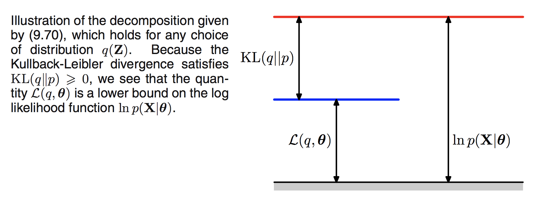
Here, the ELBO is written as $\mathcal{L}(q, \theta)$.

E-step

png

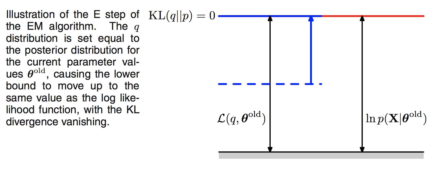
In other words, holding the parameters $\theta$ constant, minimize $\text{KL}\big(q(\mathbf{Z})\Vert p(\mathbf{Z}\vert\mathbf{X}, \theta)\big)$ with respect to $q(\mathbf{Z})$. Remember, as $q$ is a distribution with a fixed functional form, this amounts to updating its parameters $\lambda$.

The caption implies that we can always compute $q(\mathbf{Z}) = p(\mathbf{Z}\vert\mathbf{X}, \theta)$. We will show below that this is not the case for LDA, nor for many interesting models.

M-step

png

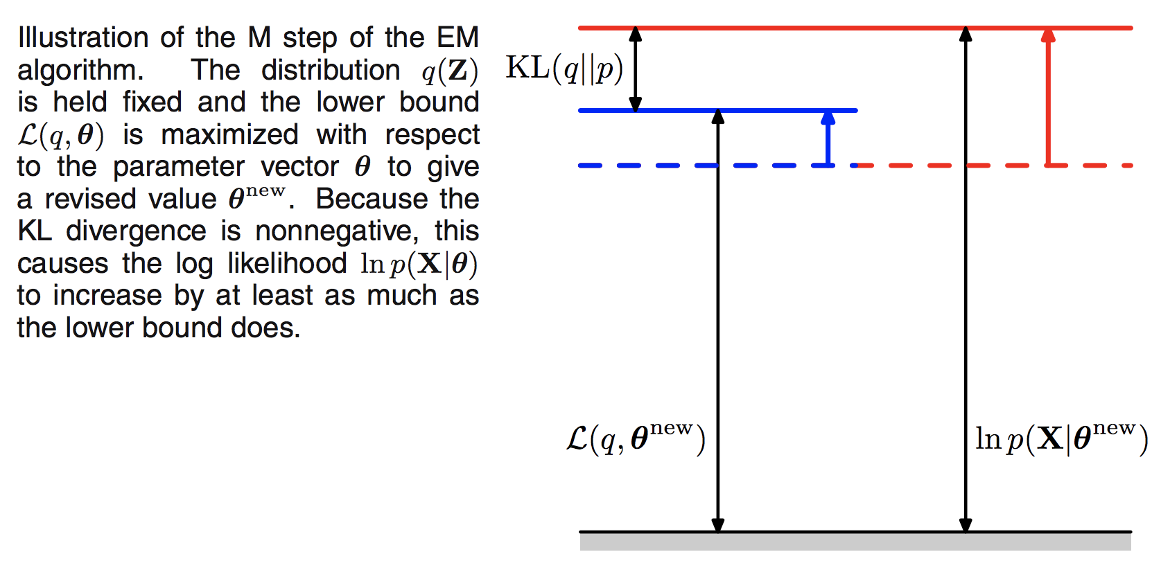
In other words, in the M-step, maximize the ELBO with respect to the model parameters $\theta$.

Expanding the ELBO:

$$ \begin{align*} \mathop{\mathbb{E}}_{q(\mathbf{Z})}\bigg[\log{\frac{p(\mathbf{X, Z}\vert\theta)}{q(\mathbf{Z})}}\bigg] &= \mathop{\mathbb{E}}_{q(\mathbf{Z})}\bigg[\log{p(\mathbf{X, Z}\vert\theta)}\bigg] - \mathop{\mathbb{E}}_{q(\mathbf{Z})}\bigg[\log{q(\mathbf{Z})}\bigg]\\ &= \mathop{\mathbb{E}}_{q(\mathbf{Z})}\bigg[\log{p(\mathbf{X, Z}\vert\theta)}\bigg] + \mathbf{H}[q(\mathbf{Z})] \end{align*} $$

we see that it decomposes into an expectation of the joint distribution over data and latent variables given parameters $\theta$ with respect to the variational distribution $q(\mathbf{Z})$, plus the entropy of $q(\mathbf{Z})$.

As our task is to maximize this expression with respect to $\theta$, we can treat the latter term as a constant.

EM for LDA

To give an example of the above, we'll examine the classic Latent Dirichlet Allocation¹ paper.

Model

png

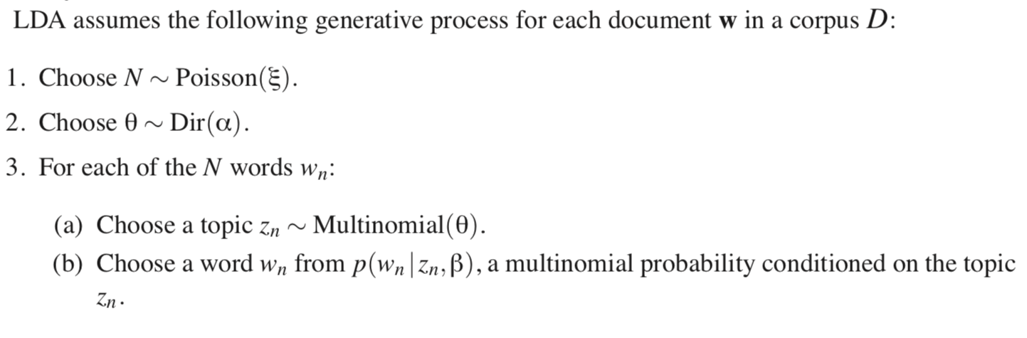
"Given the parameters $\alpha$ and $\beta$, the joint distribution of a topic mixture $\theta$, a set of $N$ topics $\mathbf{z}$, and a set of $N$ words $\mathbf{w}$ is given by:"¹

$$ p(\theta, \mathbf{z}, \mathbf{w}\vert \alpha, \beta) = p(\theta\vert \alpha)\prod\limits_{n=1}^{N}p(z_n\vert \theta)p(w_n\vert z_n, \beta) $$

Log-evidence

The (problematic) log-evidence of a single document:

$$ \log{p(\mathbf{w}\vert \alpha, \beta)} = \log{\int p(\theta\vert \alpha)\prod\limits_{n=1}^{N}\sum\limits_{z_n} p(z_n\vert \theta)p(w_n\vert z_n, \beta)d\theta} $$

NB: The parameters of our model are $\{\alpha, \beta\}$ and $\{\theta, \mathbf{z}\}$ are our latent variables.

ELBO

$$ \mathop{\mathbb{E}}_{q(\mathbf{Z})}\bigg[\log{\bigg(\frac{p(\theta\vert \alpha)}{q(\mathbf{Z})}}\prod\limits_{n=1}^{N}p(z_n\vert \theta)p(w_n\vert z_n, \beta)\bigg)\bigg] $$

where $\mathbf{Z} = \{\theta, \mathbf{z}\}$.

KL term

$$ \text{KL}\big(q(\mathbf{Z})\Vert \frac{p(\theta, \mathbf{z}, \mathbf{w}\vert \alpha, \beta)}{p(\mathbf{w}\vert \alpha, \beta)}\big) $$

Peering at the denominator, we see that it includes an integration over all values $\theta$, which we assume is intractable to compute. As such, the "ideal" E-step solution $q(\mathbf{Z}) = p(\theta, \mathbf{z}\vert \mathbf{w}, \alpha, \beta)$ will elude us as well.

In the next post, we'll cover how to minimize this KL term with respect to $q(\mathbf{Z})$ in detail. This effort will begin with the derivation of the mean-field algorithm.

Summary

In this post, we motivated the expectation-maximization algorithm then derived its general form. We then applied this framework to the LDA model.

In the next post, we'll expand this logic into mean-field variational Bayes, and eventually, variational inference more broadly.

Thanks for reading.

References

D.M. Blei, A.Y. Ng, and M.I. Jordan. Latent Dirichlet allocation. JMLR, 3:993–1022, 2003. ↩↩↩
C. M. Bishop. Pattern recognition and machine learning, page 229. Springer-Verlag New York, 2006. ↩↩↩
Wikipedia contributors. "Jensen's inequality." Wikipedia, The Free Encyclopedia. Wikipedia, The Free Encyclopedia, 29 Oct. 2018. Web. 11 Nov. 2018. ↩

Deriving Expectation-Maximization

Will Wolf