"Mean-Field Variational Bayes" (MFVB), is similar to expectation-maximization (EM) yet distinct in two key ways:
- We do not minimize \(\text{KL}\big(q(\mathbf{Z})\Vert p(\mathbf{Z}\vert\mathbf{X}, \theta)\big)\), i.e. perform the E-step, as [in the problems in which we employ mean-field] the posterior distribution \(p(\mathbf{Z}\vert\mathbf{X}, \theta)\) "is too complex to work with,"™ i.e. it has no analytical form.
- Our variational distribution \(q(\mathbf{Z})\) is a factorized distribution, i.e.
for all latent variables \(\mathbf{Z}_i\).
Briefly, factorized distributions are cheap to compute: if each \(q_i(\mathbf{Z}_i)\) is Gaussian, \(q(\mathbf{Z})\) requires optimization of \(2M\) parameters (a mean and a variance for each factor); conversely, a non-factorized \(q(\mathbf{Z}) = \text{Normal}(\mu, \Sigma)\) would require optimization of \(M\) parameters for the mean and \(\frac{M^2 + M}{2}\) parameters for the covariance. Following intuition, this gain in computational efficiency comes at the cost of decreased accuracy in approximating the true posterior over latent variables.
So, what is it?
Mean-field Variational Bayes is an iterative maximization of the ELBO. More precisely, it is an iterative M-step with respect to the variational factors \(q_i(\mathbf{Z}_i)\).
In the simplest case, we posit a variational factor over every latent variable, as well as every parameter. In other words, as compared to the log-marginal decomposition in EM, \(\theta\) is absorbed into \(\mathbf{Z}\).
becomes
From there, we simply maximize the ELBO, i.e. \(\mathop{\mathbb{E}}_{q(\mathbf{Z})}\bigg[\log{\frac{p(\mathbf{X, Z})}{q(\mathbf{Z})}}\bigg]\), by iteratively maximizing with respect to each variational factor \(q_i(\mathbf{Z}_i)\) in turn.
What's this do?
Curiously, we note that \(\log{p(\mathbf{X})}\) is a fixed quantity with respect to \(q(\mathbf{Z})\): updating our variational factors will not change the marginal log-likelihood of our data.
This said, we note that the ELBO and \(\text{KL}\big(q(\mathbf{Z})\Vert p(\mathbf{Z}\vert\mathbf{X})\big)\) trade off linearly: when one goes up by \(\Delta\), the other goes down by \(\Delta\).
As such, (iteratively) maximizing the ELBO in MFVB is akin to minimizing the divergence between the true posterior over the latent variables given data and our factorized variational approximation thereof.
Derivation
So, what do these updates look like?
First, let's break the ELBO into its two main components:
Next, rewrite this expression in a way that isolates a single variational factor \(q_j(\mathbf{Z}_j)\), i.e. the factor with respect to which we'd like to maximize the ELBO in a given iteration.
Expanding the first term
Following Bishop1's derivation, we've introduced the notation:
A few things to note, and in case this looks strange:
- Were the left-hand side to read \(\int{q(\mathbf{Z})\log{p(\mathbf{X, Z})}}d\mathbf{Z}\), this would look like the perfectly vanilla expectation \(\mathop{\mathbb{E}}_{q(\mathbf{Z})}[\log{p(\mathbf{X, Z})}]\).
- An expectation maps a function \(f\), e.g. \(\log{p(\mathbf{X, Z})}\), to a single real number. As our expression reads \(\mathop{\mathbb{E}}_{i \neq j}[\log{p(\mathbf{X, Z})}]\) as opposed to \(\mathop{\mathbb{E}}_{q(\mathbf{Z})}[\log{p(\mathbf{X, Z})}]\), we're conspicuously unable to integrate over the remaining factor \(q_j(\mathbf{Z}_j)\)
- As such, \(\mathop{\mathbb{E}}_{i \neq j}[\log{p(\mathbf{X, Z})}]\) gives a function of the value of \(\mathbf{Z}_j\) which itself maps to the aforementioned real number.
To further illustrate, let's employ some toy Python code:
# Suppose `Z = [Z_0, Z_1, Z_2]`, with corresponding (discrete) variational distributions `q_0`, `q_1`, `q_2`

q_0 = [
    (1, .2),  # q_0(1) = .2
    (2, .3),
    (3, .5)
]

q_1 = [
    (4, .3),
    (5, .3),
    (6, .4)
]

q_2 = [
    (7, .7),
    (8, .2),
    (9, .1)
]

dists = (q_0, q_1, q_2)

# Next, suppose we'd like to isolate Z_2
j = 2
\(\mathop{\mathbb{E}}_{i \neq j}[\log{p(\mathbf{X, Z})}]\), written E_i_neq_j_log_p_X_Z below, can be computed as:
def E_i_neq_j_log_p_X_Z(Z_j):

    E = 0
    Z_i_neq_j_dists = [dist for i, dist in enumerate(dists) if i != j]

    for comb in product(*Z_i_neq_j_dists):
        Z = []
        prob = 0
        comb = list(comb)
        for i in range(len(dists)):
            if i == j:
                Z.append(Z_j)
            else:
                Z_i, p = comb.pop(0)
                Z.append(Z_i)
                if prob == 0:
                    prob = p
                else:
                    prob *= p
        E += prob * ln_p_X_Z(X, Z)

    return E
- Continuing with our notes, it was not immediately obvious to me how and why we're able to introduce a second integral sign on line 3 of the derivation above. Notwithstanding, the reason is quite simple; a simple exercise of nested for-loops is illustrative.
Before beginning, we remind the definition of an integral in code. In its simplest example, \(\int{ydx}\) can be written as:
x = np.linspace(lower_lim, upper_lim, n_ticks)

integral = sum([y * dx for dx in x])

# ...where `n_ticks` approaches infinity.
With this in mind, the following confirms the self-evidence of the second integral sign:
X = np.array([10, 20, 30])


def ln_p_X_Z(X, Z):
    return (X + Z).sum()  # some dummy expression


# Line 2 of `Expanding the first term`
total = 0
for Z_0 in q_0:
    for Z_1 in q_1:
        for Z_2 in q_2:
            val_z_0, prob_z_0 = Z_0
            val_z_1, prob_z_1 = Z_1
            val_z_2, prob_z_2 = Z_2
            Z = np.array([val_z_0, val_z_1, val_z_2])
            total += prob_z_0 * prob_z_1 * prob_z_2 * ln_p_X_Z(X, Z)

TOTAL = total


# Line 3 of `Expanding the first term`
total = 0
for Z_0 in q_0:
    _total = 0
    val_z_0, prob_z_0 = Z_0
    for Z_1 in q_1:
        for Z_2 in q_2:
            val_z_1, prob_z_1 = Z_1
            val_z_2, prob_z_2 = Z_2
            Z = np.array([val_z_0, val_z_1, val_z_2])
            _total += prob_z_1 * prob_z_2 * ln_p_X_Z(X, Z)
    total += prob_z_0 * _total


assert total == TOTAL
In effect, isolating \(q_j(\mathbf{Z}_j)\) is akin to the penultimate line total += prob_z_0 * _total, i.e. multiplying \(q_j(\mathbf{Z}_j)\) by an intermediate summation _total. Therefore, the second integral sign is akin to _total += prob_z_1 * prob_z_2 * ln_p_X_Z(X, Z), i.e. the computation of this intermediate summation itself.
More succinctly, a multi-dimensional integral can be thought of as a nested-for-loop which commutes a global sum. Herein, we are free to compute intermediate sums at will.
Expanding the second term
Next, let's expand \(B\). We note that this is the entropy of the full variational distribution \(q(\mathbf{Z})\).
As we'll be maximizing w.r.t. just \(q_j(\mathbf{Z}_j)\), we can set all terms that don't include this factor to constants.
Putting it back together
One final pseudonym
Were we able to replace the expectation in \(A\) with the \(\log\) of some density \(D\), i.e.
\(A + B\) could be rewritten as \(-\text{KL}(q_j(\mathbf{Z}_j)\Vert D)\).
Acknowledging that \(\mathop{\mathbb{E}}_{i \neq j}[\log{p(\mathbf{X, Z})}]\) is an unnormalized log-likelihood written as a function of \(\mathbf{Z}_j\), we temporarily rewrite it as:
As such:
Finally, per this expression, the ELBO reaches its minimum when:
Or equivalently:
Summing up:
- Iteratively minimizing the divergence between \(q_j(\mathbf{Z}_j)\) and \(\tilde{p}(\mathbf{X}, \mathbf{Z}_j)\) for all factors \(j\) is our mechanism for maximizing the ELBO
- In turn, maximizing the ELBO is our mechanism for minimizing the KL divergence between the full factorized posterior \(q(\mathbf{Z})\) and the true posterior \(p(\mathbf{Z}\vert\mathbf{X})\).
Finally, as the optimal density \(q_j(\mathbf{Z}_j)\) relies on those of \(q_{i \neq j}(\mathbf{Z}_{i})\), this optimization algorithm is necessarily iterative.
Normalization constant
Nearing the end, we note that \(q_j(\mathbf{Z}_j) = \exp{\bigg(\mathop{\mathbb{E}}_{i \neq j}[\log{p(\mathbf{X, Z})}]\bigg)}\) is not necessarily a normalized density (over \(\mathbf{Z}_j\)). "By inspection," we compute:
How to actually employ this thing
First, plug in values for the right-hand side of:
Then, attempt to rearrange this expression such that:
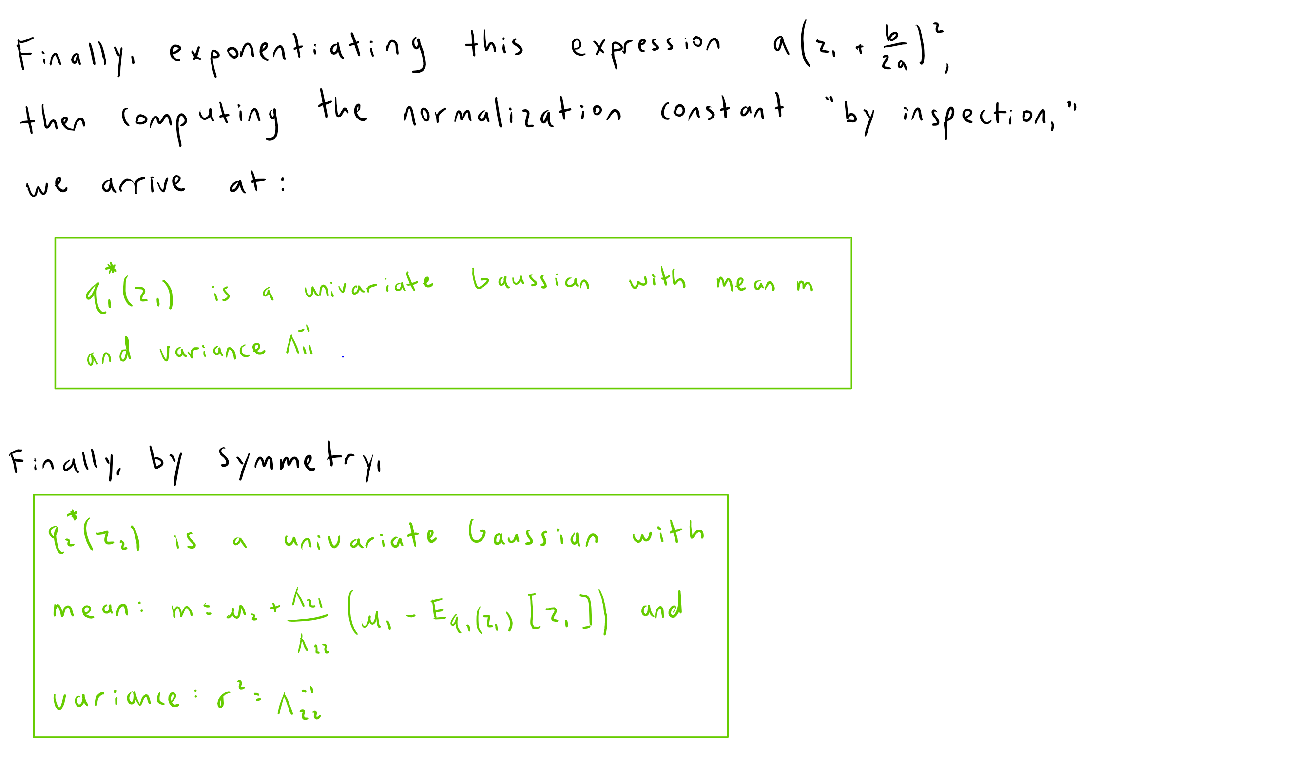
Once exponentiated, giving \(\exp{\big(\log{q_j(\mathbf{Z}_j)}\big)} = q_j(\mathbf{Z}_j)\), we are left with something that, once normalized (by inspection), resembles a known density function (e.g. a Gaussian, a Gamma, etc.).
NB: This may require significant computation.
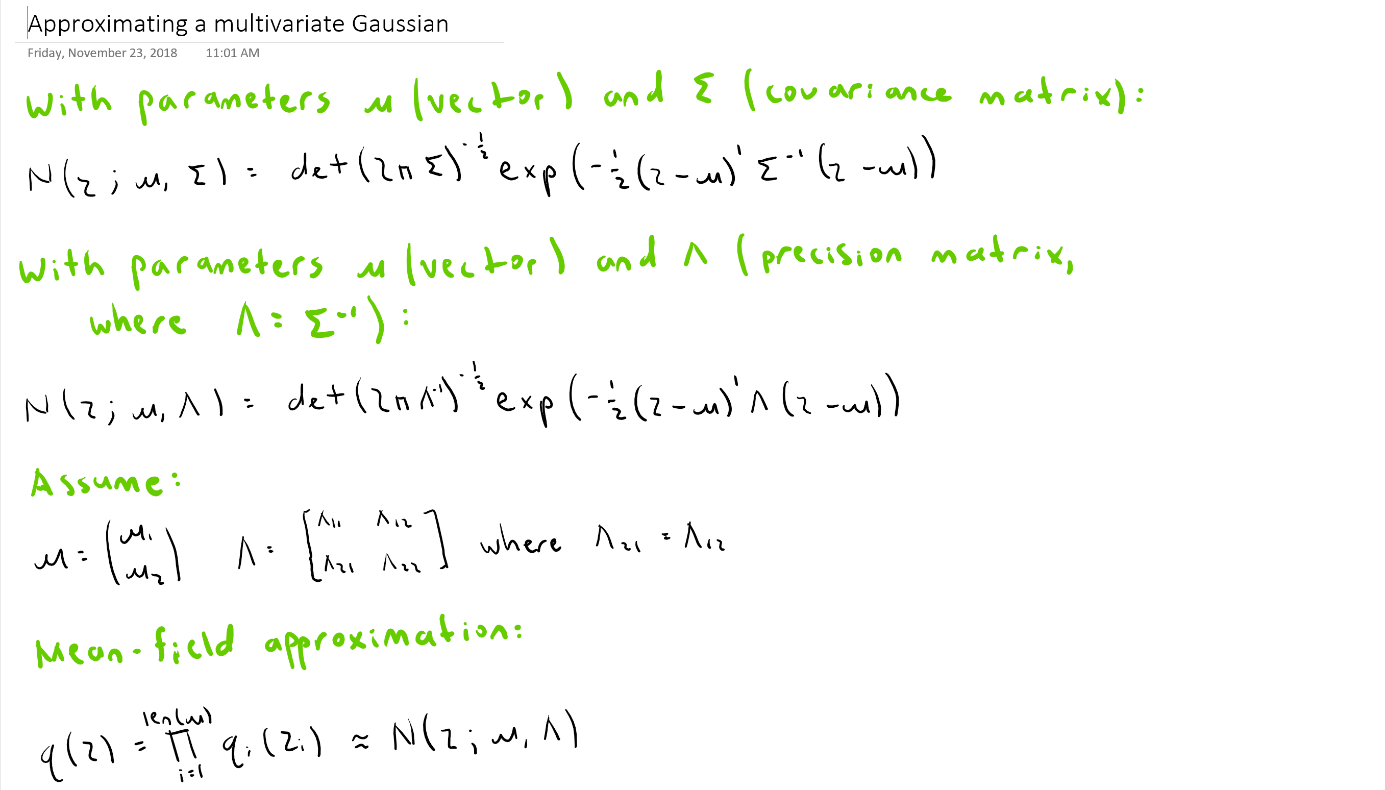
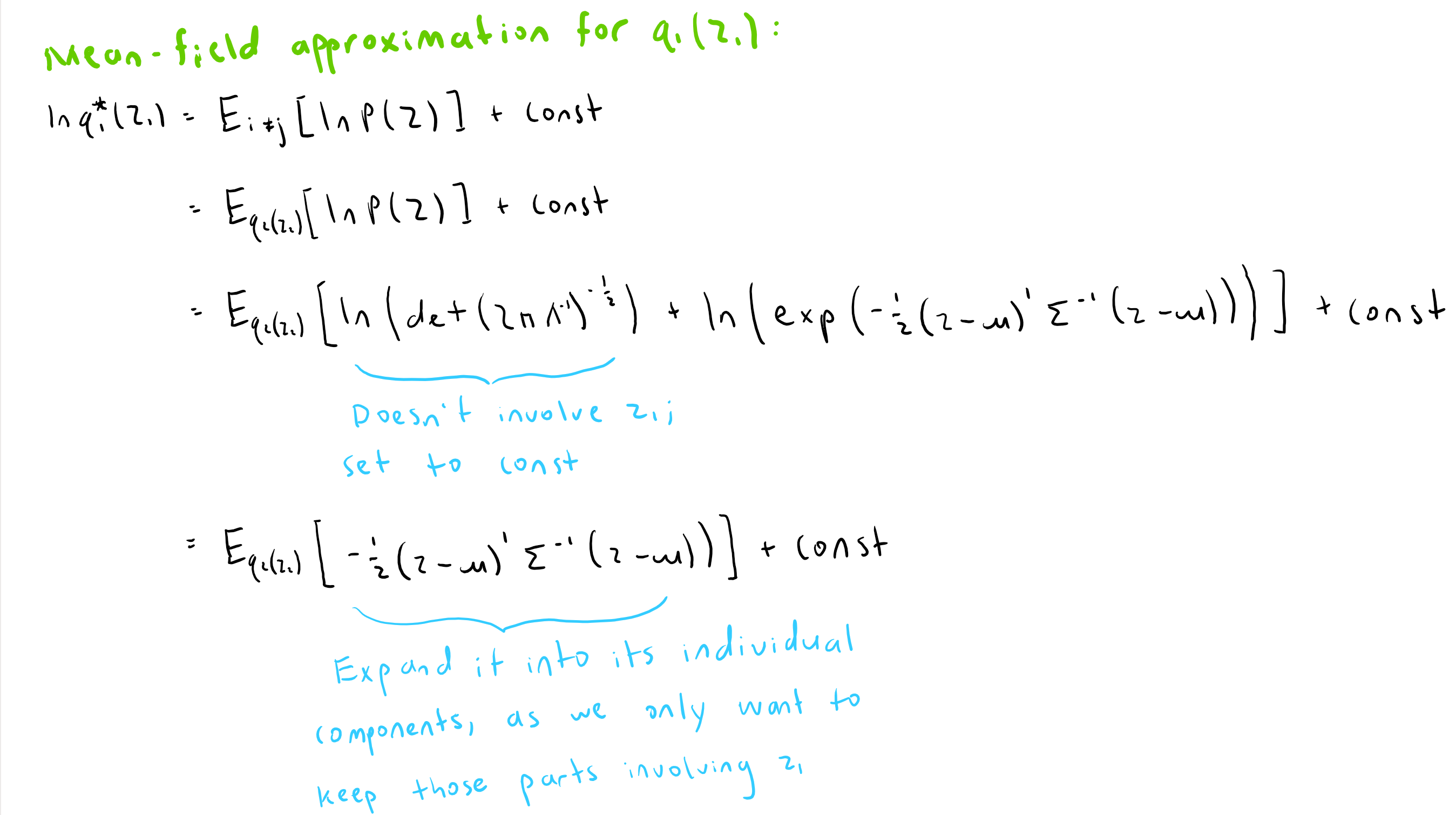
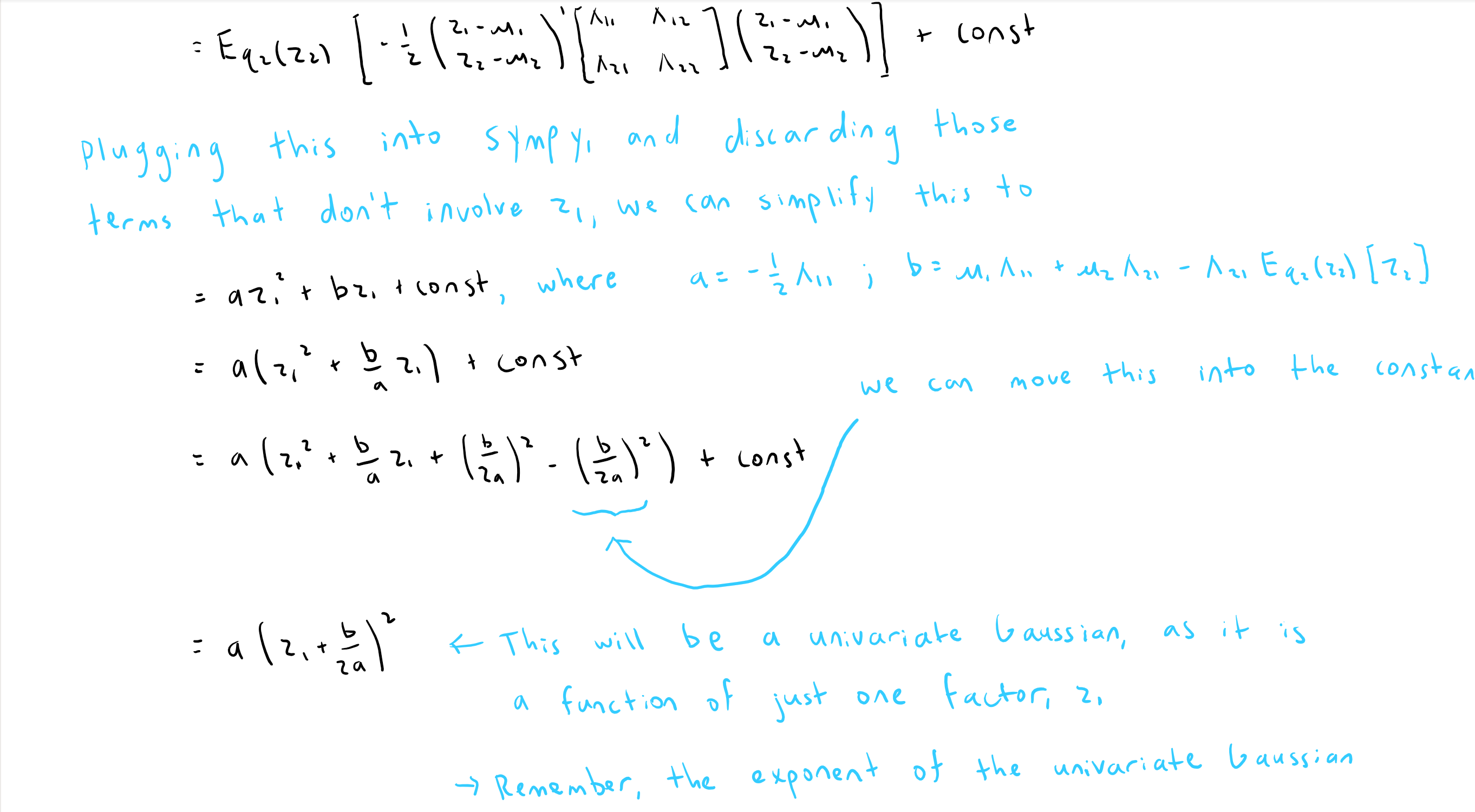
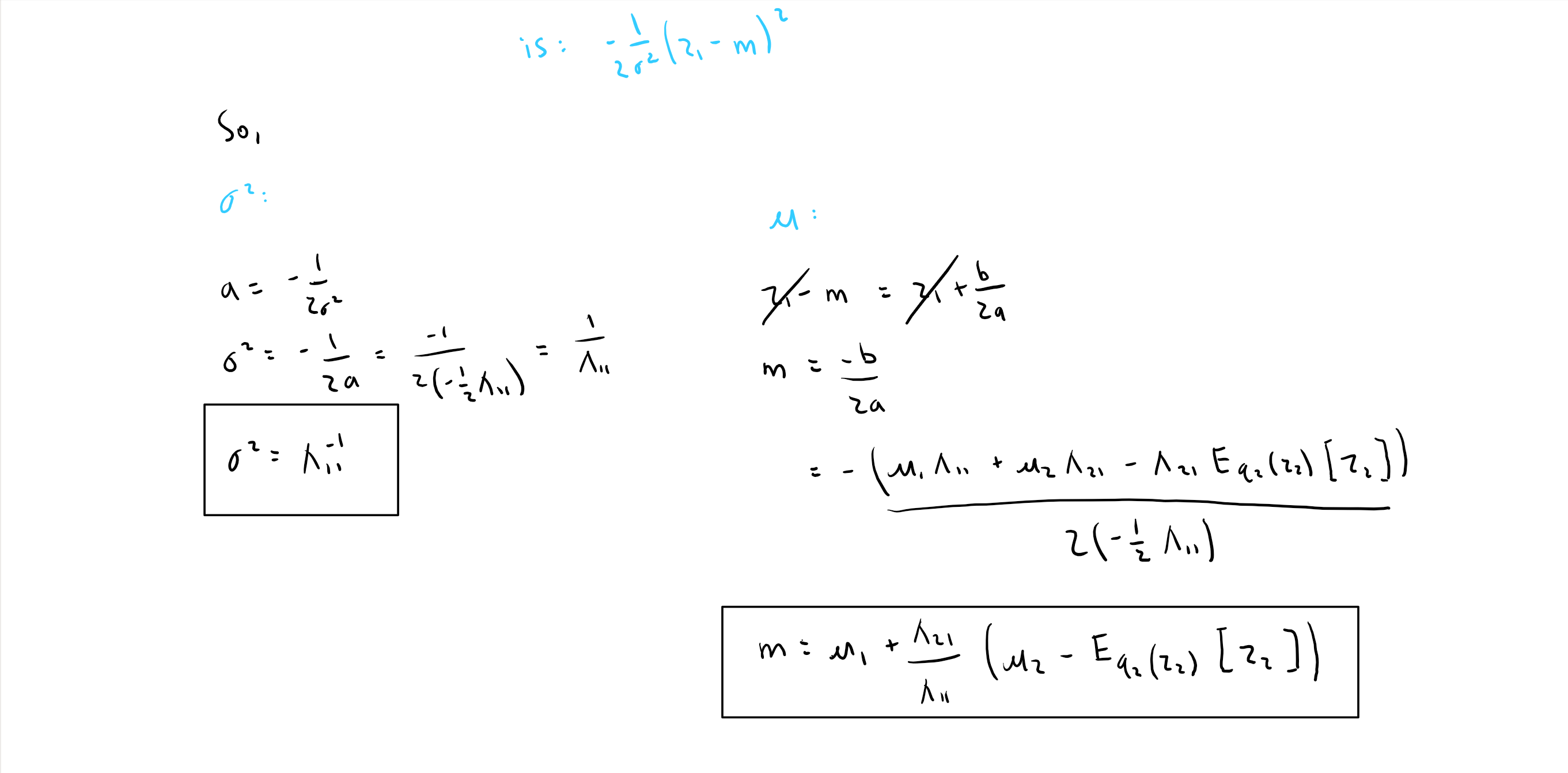
Approximating a Gaussian
Here, we'll approximate a 2D multivariate Gaussian with a factorized mean-field approximation.
Summing up
Mean-Field Variational Bayes is an iterative optimization algorithm for maximizing a lower-bound of the marginal likelihood of some data \(\mathbf{X}\) under a given model with latent variables \(\mathbf{Z}\). It accomplishes this task by positing a factorized variational distribution over all latent variables \(\mathbf{Z}\) and parameters \(\theta\), then computes, analytically, the algebraic forms and parameters of each factor which maximize this bound.
In practice, this process can be cumbersome and labor-intensive. As such, in recent years, "black-box variational inference" techniques were born, which fix the forms of each factor \(q_j(\mathbf{Z}_j)\), then optimize its parameters via gradient descent.
References
-
C. M. Bishop. Pattern recognition and machine learning, page 229. Springer-Verlag New York, 2006. ↩